To Which Family Does the Function Y=2x 5 Belong

March 02, 2022 Post a Comment

This chapter will introduce you to a particular family of functions, the trigonometric functions, which are the ground for this volume. In this first lesson, we will review the bones characteristics of functions in general: what a function is, what the graph of a office looks similar, and the characteristics of several families of functions. While this lesson will not define trigonometric functions, we will consider one of their basic characteristics, and some of import applications of these functions.

Learning Objectives [edit | edit source]

Determine if a relation is a function.
State the domain and range of a office.
Categorize a function according to a office family.
Place cardinal characteristics of functions, including the concept of a periodic function.

The Nuts of Functions [edit | edit source]

Consider ii situations shown in the boxes below:

Situation one: Your auto can travel 30 miles on one gallon of gasoline at 55 mph. For every mile per hour faster you drive, the car travels one-half a mile less per gallon of gasoline.

Situation 2: You collect data from several students in your class on their ages and their heights in inches:

Age	18	17	18	eighteen	17
Height	65"	64"	67"	68"	66"

In the first situation, let the variable x correspond the speed of your car, and let y represent the number of miles it can travel using one gallon of gasoline. If you travel at 10 miles per hour, yous will go y = 30 − .five (10 − 55) miles on one gallon of gasoline. For example, if you travel at lx mph, yous will travel 30 − .v(threescore − 55) = 27.v miles on ane gallon of gasoline. Observe that you tin use your speed to "predict" how far y'all can travel with one gallon of gasoline.

Now consider the second situation. Can yous employ the information to "predict" elevation, given the age of a student?

This is non the case in the 2d state of affairs. For case, if a student is 18 years old, there are several heights that the student could exist.

Both situations are relations. A relation is simply a relationship between two sets of numbers or data. For case, in the 2d situation, nosotros created a human relationship between students' ages and heights, just by writing each student'south information as an ordered pair. In the first situation, in that location is a human relationship between the machine'southward speed and how efficiently it tin use one gallon of gasoline. The first example is different from the second considering information technology represents a part: every x is paired with only one y. Some relations are mathematically important. For example, circles and ellipses are graphical representations of of import relations betwixt x and y coordinates, but at that place is not a unique y coordinate for each ten coordinate. Because of the unique y for each x, functions play an important office in mathematics and the science.

We tin represent functions in many ways. Some of the most common means to represent functions include: sets of ordered pairs, equations, and graphs. The figure below shows a function depicted in each of these representations:

Table one.one: Examples of functions
Representation	Example
Gear up of ordered pairs	(1,iii), (2,6), (three,ix), (4,12) (a subset of the ordered pairs for this function)
Equation	y = 3x
Graph

In contrast, the relations shown in the figure below are not functions:

Table 1.two: Examples of non-functions
Representation	Case
Set of ordered pairs	(4,2), (iv,-two), (ix,3), (9,-three) (a subset of the ordered pairs for this part)
Equation	ten = y ^two
Graph

To verify that this relation is not a function, we must show that at least one x value is paired with more than one y value. If you look at the starting time representation, the set of ordered pairs, you can run into that 4 is paired with 2 and with −two. Similarly, nine is paired with iii and with −3. Therefore the relation is not a role. If nosotros wait at the graph in a higher place, we can meet that, except for x = 0, the x values of the relation are each paired with two y values. Therefore the above relation is not a part.

One way to quickly decide whether or not a relation is a function is perform the vertical line test, which means that yous describe a vertical line through the graph. For example, if we draw the line ten = 4 through the graph of x = y ², the line volition intersect the graph twice. This means the relation is non a function.

Example 1

Determine if the relation is a part or not.

a. (ii,4), (three,9), (5,eleven), (5,12)

Solution:

a. This relation is not a function because 5 is paired with xi and with 12. If you plotted the points, the line ten = 5 would bear upon 2 points in the relation.

b. This relation is a function considering every x is paired with just one y.

In one case you are able to make up one's mind if a relation is a function, you should then be able to state the set of 10 values and the set of y values for which a role is defined.

The domain of a role is defined as the set of all x values for which the function is defined. For example, the domain of the function y = iiiten is the set of all real numbers, oft written every bit $\mathbb {R}$ . This means that x tin can exist any real number. Other functions take restricted domains. For example, the domain of the function $y={\sqrt {x}}$ is the set of all real numbers greater than or equal to zero. The domain of this function is restricted in this way because the foursquare root of a negative number is non a existent number. Therefore the domain is restricted to non-negative values of x and so that the function values will be defined.

It is oftentimes easy to determine the domain of a function by (1) considering what restrictions in that location might be and (2) looking at a graph.

Example two

State the domain of each function.

a. y = x ²

b. $y={\tfrac {1}{x}}$

c. (2, 4), (3, 9), (5, 11)

Solution:

a. The domain of this function is the set of all real numbers. In that location are no restrictions.

b. The domain of this function is the set of all real numbers, except ten ≠ 0. The domain is restricted this way because a fraction with denominator zippo is undefined.

c. The domain of this function is the fix of x values {2, three, v}.

The variable x is ofttimes referred to as the independent variable, while the variable y is referred to every bit the dependent variable. Nosotros talk about x and y this way because the y values of a function depend on what the x values are. That is why nosotros also say that "y is a function of x". For instance, the value of y in the office y = 310 depends on what x value we are considering. If x = iv, nosotros can easily decide that y = three(iv) = 12.

When nosotros are working with a function in the form of an equation, at that place is a special annotation we tin can utilise to emphasize the fact that y is a function of x. For example, the equation y = three10 tin can besides be written equally f(x) = 3x. Information technology is important to remember that f(x) represents the y values, or the function values, and that the letter f is not a variable. That is, f(10) does not hateful that nosotros are multiplying a number f past another number 10. Retrieve of a role as a car that takes in a number, x, and produces another number. In the expression f(10), f is the machine and the parenthesis () are the identify where the input, x, is entered into the automobile. f(x) is the output that the automobile produces with the input 10. For example, consider that your machine adds 5 to an input. So f(3) = 8, or more generally, f(x) = x + 5.

Now that we have considered the domain of a function, we will turn to the range of a function, which is the set of all y values for which a office is defined. Just as we did with domain, we tin examine a function and determine its range. Once again, it is frequently helpful to think about what restrictions there might be, and what the graph of the function looks like. Consider for example the part y = ten ². The domain of this function is all real numbers, but what about the range?

The range of the function is the fix of all existent numbers greater than or equal to nothing. This is the case because every y value is the square of an x value. If nosotros square positive and negative numbers, the result will always exist positive. If x = 0, then y = 0. We tin also see the range if we expect at a graph of y = x ²:

Some functions have sudden jumps. Consider the "rounding" function that takes a number and rounds it to the nearest whole number (rounding upwardly if the number is exactly between ii whole numbers). Then some values for this office are (two, 2), (1.4, ane), (3.9, 4), (five.5, 6), and (−5.5, −five). The domain of this function is all real numbers, only the range of the function is the integers.

Some other function that jumps comes from the way taxis frequently charge. Suppose a taxi costs $5.00 for the first 2 miles only and then $i for each additional mile or fraction of a mile. Consider the part that has the distance traveled as the input and the cost of the taxi ride as the output. So some values for this role are (1, v), (1.9, 5), (2.i, six), (10, thirteen). The domain of this function is the non-negative real numbers (since you tin't travel a negative altitude in a taxi cab). The range of this function is all positive integers greater than or equal to 5: {5, 6, seven, 8, ...}.

Case three

Country the domain and range of the role $y={\tfrac {2}{x}}$

Solution:

For this function, we tin can choose whatever x value, except 10 ≠ 0. Therefore the domain of the role is the set of all real numbers, except x ≠ 0.

The range is too restricted to the non-goose egg real numbers, only for a different reason. Considering the numerator of the fraction is 2, the numerator tin never equal zippo, and so the fraction tin can never equal zip.

At present that we take divers what it means for a relation to exist a office, and nosotros have divers domain and range of a office, we can look at some specific examples of functions and their graphs.

Families of Functions [edit | edit source]

The examples we have seen and then far accept included several unlike types of functions. From your previous feel working with equations and graphs, you lot may have already made connections between the forms of the equations of functions, and what the graphs look similar. Hither we will examine several "families" of functions. A family of functions is a set of functions whose equations have a similar grade. The "parent" of the family unit is the equation in the family with the simplest form. For example, y = x ² is a parent to other functions, such as y = 2x ² − vx + iii. The table below summarizes the key aspects of several families of functions.

Tabular array 1.3: Families of functions
Family unit	Parent(s)	Key aspects
Linear	y = x	The graph of a linear function is a straight line, which is often identified in terms of its slope and its y-intercept. The slope of the line is the coefficient ${\tfrac {i}{2}}$ , and the y-intercept is the constant ane.
Quadratic	y = ten ^two	These functions have a highest exponent of 2. The graph is a parabola, which has a vertex that is either a global maximum or minimum of the graph. The vertex is the point (1, -ane). The graph is symmetric across the line 10 = 1.
Cubic	y = x ⁱⁱⁱ	These functions accept a highest exponent of 3. The ends of the graph accept opposite behavior. Cubic graphs either have a local maximum and minimum, like the one in the graph to the right, or no local maximums or minimums, like y = x ³.
Exponential	y = 2^x, y = iii¹⁰, etc.	Exponential functions have a variable as an exponent. The graph has a horizontal asymptote. Every bit x approaches $-\infty$ , the part values approach the x−axis (y = 0).
Rational	$y={\tfrac {1}{x}},$ etc.	These are functions that contain fractions with polynomials in the numerator and denominator. The graphs have a horizontal and a vertical asymptote. Every bit x approaches $\pm \infty$ , the y values arroyo 0 (the x−axis). As x approaches 1, the y values arroyo $\pm \infty$ .

All of these functions can be used to represent real situations. For example, the linear function y = 3x was used in a higher place to represent how much money you would make selling candy confined for $3.00 each. This type of situation is known equally direct variation. We say that the corporeality of money you make varies direct with the number of candy bars you sell. Straight variation between two variables will always be modeled with a linear part of the grade y = mx. The gradient of the line, grand, is the constant of variation. Notice that the y−intercept of the line is 0; that is, the line contains the point (0, 0). This makes sense in terms of the processed selling state of affairs: if you sell 0 processed bars, y'all make 0 dollars.

Other situations can be modeled with a unlike kind of linear function. Consider the following situation: a restaurant is having a special: a large cheese pizza costs $8.00, and each topping costs $2.00. The cost of a pizza tin can be modeled with the function c(x) = 2x + 8, where x is the number of toppings on the pizza. The slope of the line is ii, every bit each topping adds $2 to the price. The y−intercept is 8: if you practice not cull whatever additional toppings, the pizza costs $8.00.

Quadratic, cubic, and other polynomial functions tin exist used to model many types of situations Another of import family unit of functions is the rational functions, or quotients of polynomials, such as:

f(ten)={\frac {3x}{x^{2}+one}}

f(x)={\frac {1}{x}}

For example, a rational function is used to model changed variation between 2 variables. Changed variation means that the product of ii variables is abiding: xy = k. If we solve this equation for y, we have $y={\tfrac {k}{x}}$ , a rational function. The post-obit example shows inverse variation in a real situation:

Example 4

Some days y'all drive to work, and other days you ride your bike. Yesterday you collection at an average rate of 40 miles per hour, and it took fifteen minutes. Today you lot rode your bike a charge per unit of twenty miles per hour, and it took half an hour.

Write an equation that shows the human relationship between your speed and the fourth dimension it takes to go to work.

Solution:

y={\frac {10}{10}}

, where x is your speed in miles per hour and y is the time it takes to go to work in hours.

First, note that the distance betwixt home and piece of work is 10 miles:

{\text{twoscore miles per hour}}\times {\frac {one}{4}}hr={\text{ten miles}}

{\text{twenty miles per hour}}\times {\frac {1}{2}}hr={\text{10 miles}}

Nosotros know that in general:

{\text{charge per unit}}\cdot {\text{fourth dimension}}={\text{distance}}

{\text{time}}={\frac {\text{altitude}}{\text{rate}}}

Therefore if you bulldoze or ride at a rate of 10 miles per hr, it will accept you y hours to get to piece of work: $y={\frac {x}{x}}$ .

In full general, functions can be used to model existent phenomena in many contexts, including unlike areas of science, business, economics, and more. The blazon of function that can exist used to model a specific situation depends on the central aspects of a office that will lucifer central aspects of the state of affairs. 1 attribute of many situations is not seen in the function types we take seen and then far, but will be seen in the trigonometric functions you will learn about in this affiliate. Consider for instance, the table below, which shows the average monthly high and low temperatures in the urban center of Boston, MA, from 1971 to 2000. (Source: rssweather.com)

Tabular array 1.four: Average monthly high/low temperatures for Boston, MA
Month	Low	High
January	22.one°F	36.5°F
February	24.2°F	38.7°F
March	31.5°F	46.3°F
April	40.5°F	56.1°F
May	l.2°F	66.7°F
June	59.iv°F	76.6°F
July	65.five°F	82.2°F
August	64.5°F	lxxx.1°F
September	56.8°F	72.5°F
October	46.four°F	61.8°F
Nov	37.nine°F	51.8°F
December	27.8°F	41.seven°F

The graph below shows the average low temperatures.

Detect that the graph includes a full year of data, and then ends with December, the 12^th month. It is possible that the bend suggested by this graph can be approximated past a function in one of the families of functions nosotros've discussed. Not all natural phenomena tin can exist modeled with mathematical functions, but many tin can.

Suppose this information was representative of Boston weather condition in general. Nosotros could make a function whose input is the time in months from the present and whose output is the average temperature expected. For example f(1) = 22.1, f(v) = 50.2. The function will echo later ane twelvemonth. What does 13 represent? What is the temperature expected to be based on this information?

Because the months cycle each year, 13 represents January of the side by side year, and in full general, we tin predict the weather in January given our knowledge of the usual climate in a location. For instance, Jan is the coldest month of the twelvemonth in the urban center of Boston. For the years shown in the table, the average low temperature was most 22 degrees. Nosotros can therefore predict that the boilerplate low temperature in January in Boston will exist about 22 degrees. We could use such a office to compare current weather to by weather and examination for climate changes over fourth dimension.

Because the months of the year and the weather condition patterns are cyclical in nature, nosotros need to model this situation with a function that is also cyclical in nature. Such functions are referred to as periodic. A function is periodic if there exists some value p such that f(x + p) = f(x) for all x in the domain of the function. The trigonometric functions you volition learn most in this chapter are one blazon of periodic function, and we can utilize certain trigonometric functions to model the conditions information shown above. We will return to this topic at the end of this lesson, but now we will look at the graphs of functions.

Graphing Functions and Technological Tools [edit | edit source]

While there are techniques you tin can utilise to efficiently graph many functions by hand, using a graphing calculator allows you to quickly graph any function, and to identify fundamental aspects of the function. The following two examples volition show you how to use a TI graphing calculator to explore a part.

Instance 5

Graph the function y = ten ³ − 3x ² + 1

a. Evaluate the function for x = 0, x = two, and x = −2.

b. Describe the end behavior of the function.

c. Estimate all x−intercepts.

d. Estimate whatsoever local maxima and minima.

Solution:

To graph this function, press [Y=], and articulate any equations already entered. In Y1, enter the equation. If you have never entered an equation before, here are some tips:

The x button is correct next to the green [Blastoff] button (on the TI-83 model).
To enhance 10 to the 3^rd power, press [MATH].
To raise 10 to the second power, press the [ten²] button, which is in the left column.
Exist careful with negatives: the blue "−" button on the correct side is for subtraction. The button on the bottom that says "(−)" is for negative numbers.

In one case y'all accept entered the equation, press [ZOOM] [vi]. This volition have yous to the "standard" window: you can see both 10 and y from −10 to ten. (Note that if you scroll downward to option 6, you have to press enter. Nevertheless, if you simply enter the number 6, yous will be taken to the graph.)

a. To evaluate the function, y'all can "trace" on the graph. Press the [TRACE] push. You should see the equation at the meridian of the screen, and the cursor should be on the y-intercept, (0, i). At the bottom of the screen you should run across x = 0 and y = 1.This tells us that for x = 0, the role value is one.

Now that y'all are in tracing style, y'all can enter any x value, and the reckoner will tell yous the y value. For example, if you lot press [2] [ENTER], yous will meet the cursor movement to the point (2,−3) and at the bottom of the screen, you lot will see x = ii and y = −3. If you press [(-)] [2] [ENTER], yous will run into x = −2 and y = −19 at the lesser of the screen. Find that you cannot see the point on the graph. To meet that point, nosotros need to alter the window. Press [WINDOW] and roll down to Ymin. Change the −10 to −25. Then press [GRAPH]. Now press [TRACE] [(-)] [2] [ENTER]. You should see the point (−two,−19).

b. End behavior: the left-hand side of the graph appears to be going down, and the correct-hand side appears to be going up. If we want to see more than of the graph, we can zoom out. Press [ZOOM] [iii]. This will increase the size of the window. If y'all press [ENTER] again, the window will increase once more. If you exercise this twice, you will notice that the axes expect thick and that the graph is hard to see. This is because the tick marks on the axes are set up in 1s. Press [WINDOW] and scroll down to Xscl. If you lot press [DELETE], this volition remove all tick marks. (You tin can also set the calibration to something larger.). To run across the graph better, you can besides reduce the Xmin and Xmax. Set Xmin to −20 and Xmax to 20. Printing [GRAPH]. Now y'all can see the part. Printing [TRACE] in either direction, and y'all will be able to see that the left-manus side of the graph continues going down, and the right-hand side continues going upwardly.

c. The x−intercepts: to return the graph to a smaller window, press [ZOOM] [vi]. If you want to see the graph in a smaller window, press [ZOOM] [4]. You should encounter that the graph has iii x−intercepts. Y'all can visually estimate them by tracing: press [TRACE] and move the cursor left. The leftmost 10−intercept is around −.5. To discover a skilful approximation of the x−intercept, press [2nd] [TRACE] [ii]. This sends you back to the graph. On the screen you will see the question "Left bound?" Motility the cursor to the left of the 10−intercept. (You volition be moving down, in this case.) Press [ENTER]. Then you volition see the question "Correct bound?" Move the cursor to the right of the x−intercept, merely don't go also far (Yous don't want to pass the next x−intercept.) Press [ENTER]. So yous will be asked to "guess" the intercept. Move the cursor dorsum to the left, as shut to the 10−intercept as possible. Press [ENTER]. You should see x = −.5320888. This is an approximation of the x−intercept. If you use the use same steps, you volition observe that the other x−intercepts are approximately .6527 and two.879.

d. Maxima and minima: notice that the graph as a "hill" and a "valley". The hill is called a "local maximum" because information technology is the highest indicate on the graph, within a certain interval. The valley is similarly a "local minimum". To judge the coordinates of the maximum, press [TRACE] and trace close to the maximum. Information technology appears that the maximum is (0, ane). To verify this, printing [2nd] [TRACE] [4]. To find the maximum, we have to do the same "left bound, right bound, guess" process nosotros used to observe the ten−intercepts. This process should tell you that the maximum is (0, 1). (Note: the ten value may say something like "9.64487Eastward −7." This is just a minor calculator error. This number is very close to 0!) To find the minimum, trace towards the "valley". (If you want, you can become to the [WINDOW] and make the Ymin a lower number, so that you can clearly see the minimum of the graph.) Now press [2d] [TRACE] [3]. This will bring you dorsum to the graph. Doing the "left spring, right bound, guess" process should show you that the minimum bespeak is (two, −3).

Case vi

You have 100 anxiety of fence with which to enclose a plot of state on the side of a barn. You desire the enclosed land to be a rectangle.

a. Write a function to model the area of the plot as a office of the width of the plot.

b. Graph the function using a graphing calculator.

c. What size rectangle should you make with the fence in lodge to maximize the expanse of the rectangular enclosure?

d. Explain the significance of the x−intercepts.

Solution:

The plot of state volition look like the picture below:

a. The equation: The area of the rectangular plot is the product of its length and width. Nosotros can write the surface area as a function of x: A(x) = 2xh. Nosotros tin can eliminate h from the equation if we consider that we take 100 feet of argue, and nosotros write an equation about how we are using that 100 feet of fence: x + twoh = 100. (The fourth side of the rectangle does not crave fence because of the barn.) We tin can solve this equation for h and substitute into the area equation:

b. The graph: Press [Y=] and clear whatever equations. Then enter the equation in Y1. Notice that if yous press [ZOOM] [6], y'all will not see whatever graph. Yous tin zoom out by pressing [ZOOM] [iii], but it may be more efficient to cull a window based on function values. Press [2nd] [WINDOW] in gild to set up the tabular array. TblStart is the first entry yous want to see in the table. Tbl allows you lot to gear up the increments. For example, if you lot want to see x = i, 2, 3, iv, etc, set this to 1. For this example, set up this to x. Make sure Indpnt and Depend (10 and y) are set to "auto". Then press [2nd] [GRAPH] to encounter the table. If you scroll through the table, you will see that the y value reaches 2500 at x = 50, and and so the values decrease. Now nosotros tin ready the window. Press [WINDOW]. and set Xmin = −one, Xmax = 105, Ymin = −200, and Ymax = 3000. (Note: you can prepare Xmin and Ymin each to 0, simply setting them at −1 and −200 allows y'all to meet the axes.)

The graph of A(x) is shown here on the interval [0, 100].

c. The maximum possible area: using the process from example 6, you should detect that (fifty, 2500) is the maximum point. This tells us that when the rectangle's width is 50 ft, the area is 2500 ft².

d. Intercepts: Using the process from example 5, you should find that the 10 intercepts are at 0 and 100. This tells us that if the width of the garden is 0, so the area is 0. If the width of the plot of land is 100, then the area is 0. This is the instance because there is only 100 feet of argue. If the width is 100, there is no more than fence for the rest of rectangle!

Introduction to Trigonometric Functions [edit | edit source]

Consider again the temperature data from above:

As was noted above, this kind of data needs to be modeled with a role that is periodic. In particular, this kind of data is ofttimes modeled past a sinusoid, a graph that oscillates in a particular mode, as seen in the graph beneath.

Every sinusoid repeats its values on a regular interval. If we modeled the weather condition data with such a graph, the values will repeat every 12 months. Therefore nosotros say that the period of the function is 12.

Notice that the information ranges from about 22 to 65. Also notice that the "moving ridge" centers in between these values, around y = 43. Therefore we say that the amplitude of the wave is about 21, which is the distance from the middle to the top or the bottom of the wave.

Many existent phenomena tin can be modeled with this kind of office.

Lesson Summary [edit | edit source]

In this lesson we take reviewed the concept of a function, including major aspects of functions, and dissimilar types of functions. We take also used graphing calculators to graph and explore different functions. A key point of this lesson is that we can use functions to model real phenomena. A second cardinal indicate is that in order to model phenomena that are cyclical in nature, nosotros need to use functions that are periodic. In lesson 4 in this chapter we will ascertain six trigonometric functions. However, considering the inputs of these functions are angles, in the next 2 lessons we will focus on angles. First we will review angles in triangles from Geometry, and then we will consider angles in rotation.

Points to Consider [edit | edit source]

What distinguishes a part from a relation?
What makes a function periodic?
What are the pros and cons of using a calculator to graph a function?

Review Questions [edit | edit source]

Determine if each relation is a function:

(a) (−one, 4), (0, three)(1, 5), (one, 7), (2, 15)

(b) y = 3 - x

(c)
A train travels at a constant speed of 95 miles per hour.

(a) Write an equation that shows the relationship betwixt the number of hours the train has traveled and the distance it has traveled.

(b) Is this situation direct variation, inverse variation, or neither?

(c) Use the equation to determine the distance the train has traveled after 3 hours.
You lot decide to offset a modest business organisation making picture frames. You spend $100 on pigment and other supplies, as well as $ii.00 per wooden frame. Yous decide to sell each frame for $10.00.

(a) Write a linear function that models the costs of your business organization.

(b) Write a linear function that models the acquirement of your business organisation. (Acquirement is the amount of money you take in.)

(c) Write a linear function that models the profits of your business. (The profits can be constitute by subtracting the costs from the acquirement.)

(d) Use your profit function to determine the minimum number of frames that must exist sold to make a profit.
Consider the function defined past the equation f(x) = x ² − x − 3.

(a) To what family does this office belong?

(b) Country the domain and range of the role.

(c) Use a graphing calculator to graph the function, to place the approximate coordinates of the vertex, and the approximate values of the x−intercepts.
Consider the function $y={\tfrac {10-two}{ten+3}}$

(a) Utilize a graphing reckoner to graph the office.

(b) Identify all asymptotes.
The price of reserving a private party room in a restaurant is $500. The price per person varies inversely with the number of people who nourish the political party.

(a) Write an equation that represents the relationship between c, the cost per person, and p the number of people attention.

(b) Use the equation to detect the cost per person if 32 people attend.
Use a graphing calculator to graph the functions y = x ³ + 10, y = x ^three + 2ten, y = x ³ − x, and y = x ^three − 2ten. What is the consequence of irresolute the coefficient on the second term?
The equation p(x) = −.510 ² + 90x − 200 represents the profits of a visitor, where ten is the number of units the company sells. Apply a graphing calculator to graph the function, and use the graph to respond the questions.

(a) What is the maximum profit, and how many units must be sold to reach the maximum turn a profit?

(b) Find the x−intercepts and explain the pregnant of these points on the graph in terms of the profits of the company.
The table below shows the average daylight hours each calendar month in Anchorage, Alaska.

(a) Use your graphing reckoner to plot the data, or graph by mitt. Use January = 1.

(b) What is the menstruation of the data?

(c) How might the graph expect different if the data represented daylight hours where y'all live?

Table 1.5
Month	Average daylight hours
Jan	5.65
February	7.77
March	x.4
April	13.37
May	sixteen.87
June	18.72
July	19.xviii
Baronial	17.12
September	fourteen.27
October	11.43
November	eight.53
December	6.xiii

Review Answers [edit | edit source]

(a) Not a function

(b) Is a function

(c) Not a role
(a) y = 95x

(b) The situation is directly variation.

(c) 285 miles
(a) C(x) = 2ten + 100

(b) R(x) = tenten

(c) P(x) = viiiten - 100

(d) You must make and sell 13 frames to make a profit.
(a) This is a quadratic function.

(b) The domain is the set of all real numbers. The range is the set of all real numbers greater than or equal to three.25.

(c) Vertex: (.5, -3.25); ten-intercepts: -one.3, 2.3
(a)

(b) 10 = -3, y = 1
(a) $cp=500\quad {\text{or}}\quad c={\frac {500}{p}}\quad {\text{or}}\quad p={\frac {500}{c}}$

(b) $fifteen.63
The equations with positive coefficients await more and more similar y = 10 ³, every bit the coefficient gets larger. The equations with negative coefficients take local maxes and mins. Decreasing the coefficient increases the size of the "hill" and the "valley".
(a) Maximum profit is $3,850, with ninety units sold.

(b) 2.25 and 177.75. These are the pause-even points. When 2−three units are sold, the company has made enough coin to brand up for initial costs. After selling 177 units, the company is no longer profitable.
(a)

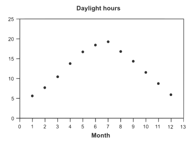
(b) Catamenia = 12

(c) In other U.S. cities, the daylight hours do not vary and so profoundly. The amplitude of the graph would be smaller.

Vocabulary [edit | edit source]

dependent variable: The input variable of a function, usually denoted x.
domain: The domain is the fix of input values (x) for which a office is defined.
function: A relation in which every chemical element of the domain is paired with exactly 1 element of the range.
independent variable: The output variable of a role, usually denoted y.
periodic office: Any office that repeats regularly.
range: The set of output or office values (y) for a function.
relation: A pairing betwixt the items in two sets of numbers or information.; COODINATES is two points in the graph or function;

← Trigonometry and Right Angles · Angles in Triangles →

This material was adapted from the original CK-12 book that can be institute here. This work is licensed under the Creative Commons Attribution-Share Alike 3.0 United States License

robinsonlinto1947.blogspot.com

Source: https://en.wikibooks.org/wiki/High_School_Trigonometry/Basic_Functions